
Thursday
Oct152009
How Low Can You Go? Using Simulation to Determine Appropriate Inventory Levels
 NOTE: We wrote this article years ago for a lean conference. We stumbled upon it recently and found that it is still relevant today. Though it refers specifically to the manufacturing sector, there are lessons here for all sectors.
Proper inventory levels are critical to maximizing your manufacturing system’s performance; but what level of inventory is best? Too much inventory will add cost and increase cycle time. Too little inventory will jeopardize total output. Achieving good system performance depends upon a very difficult and often non-intuitive exercise in balancing capacity against demand. This exercise is made all the more difficult by the random variability inherent in any real system. Fortunately, there is a tool – discrete event simulation - that gives you the very valuable ability to understand how variability and randomness affect your process. Perhaps most importantly, however, simulation allows you to experiment with various inventory policies in determining the best balance for your particular system, all without having to implement non-optimal choices in the real system.
After a review of basic issues in inventory management, we provide an overview of simulation in this context. We will discuss simple simulation examples as well as case studies from manufacturing, service, and supply chain analysis. We conclude by offering advice for implementing simulation in your organization.
Introduction
Inventory, for our purposes here, is defined as a collection of any item or resource used in an organization to produce manufactured goods. We will look at five types of inventory that are commonly addressed by lean initiatives: raw materials, work-in-process, finished goods, production capacity, and labor. Once the purpose of inventory is understood, we can then make efforts to minimize inventory which will in turn help to improve production cycle times and lower inventory.
As an analytical planning tool, simulation naturally lends itself to lean analysis. Simulation mimics the dynamics and randomness of manufacturing processes. This variation is the main reason inventory exists in most systems. Through the proper use of simulation technology, organizations can determine the lowest levels of inventory required to absorb the variability found within any system.
Purpose of Inventory
Variation in all its forms is the source of inventory build-up in virtually all systems. Not all inventory build-up is negative, and is in fact an effective means of coping with variation itself. In this section, we review the specific ways in which inventory may arise from variability in everything from raw material prices to production speeds.
Raw Materials
Raw materials feed the system and keep it moving. Without it, production must eventually stop. On the other hand, excess raw materials can strain the inventory holding capacity of the system as a whole. As with all else, finding the right balance is key. The idea is to have the lowest level of inventory that will still allow you to meet your objectives. The following is a list of the reasons for holding inventory.
Take Advantage of Ordering in Economic Quantities (Volume Discounts)
In many cases, there may be substantial savings when raw materials are ordered in larger quantities than may be immediately required in production. These savings must be balanced against the costs of holding the resulting raw materials inventory.
Provide a Safeguard Against Variable Lead Times And Quality
 In order for the production process to continue smoothly, raw materials must be available when needed by the system. This is not always as simple as it sounds, however, as materials often come from independent vendors. If the raw materials have a variable ordering lead-time, it is wise to hold some additional inventory as a hedge against those cases in which the ordering lead-time may be longer than expected. A related concern may occur when the raw materials supplied may vary in quality. If a larger-than-expected portion of the raw materials must be rejected on the basis of quality, a stock-out could occur. Again, a company may choose to hold a bit of additional inventory of this material as a safeguard.
Price Speculation
As with most other elements of a system, the price of raw materials may be highly variable. In such cases, it is often common practice to ‘stock-up’ on raw materials that are currently at a low point on their price scale. This practice, while economically favorable, can lead to excess raw material inventory.
Work-in-Process
Some level of work in process is a desirable element in many systems, and may arise for a variety of reasons. The most principal of those reasons are discussed below.
Buffer Variability in Production Rates
Consider two sequential operations each working at different rates and with different degrees of variability. With no Work-in-Process (WIP) buffer between the operations, the second operation would be highly dependent on the output of the first operation. If the first operation is significantly slower, or is experiencing an unusually slow processing time, the second operation is blocked. Similarly, if the first operation finishes an item before the downstream operation is ready to accept it, the first operation must stop working until it can pass on the completed item. Including a buffer between these two operations to accumulate WIP allows for the operations to continue operating independently.
Allow for Flexibility in Production Scheduling
Changeovers that result when one product type follows another may be a significant aspect of the system’s overall performance. In such cases, it is often possible to minimize the effects of changeovers through clever production scheduling. The more product types that are available in WIP inventory at each stage of the production, the more options there are for production scheduling. As a result, WIP is sometimes deliberately built in to allow for this flexibility.
Absorb Different Labor Shift Patterns
Variations in labor availability can be caused by many factors, such as seasonal increases in demand, or shortages due to strike. Keeping some additional WIP around labor-critical phases of the production can be instrumental in absorbing the effects of variation in labor availability.
Absorb Unexpected Equipment Down-Times
Everything breaks eventually. Murphy’s law, of course, says that equipment will go down at the most inopportune time. Maintaining WIP inventory of the product produced by the more unreliable operations will allow both upstream and downstream operations to continue while the machine is being repaired.
Finished Goods
Most manufacturers ideally like to sell all inventory as fast as it is produced. At the same time, good customer service typically dictates that no customer should be made to wait for a product. After all, the customer may simply decide to go down the street to your competitor if you do not have the goods available. The compromise between these situations typically involves some amount of finished goods inventory.
Provide a Safeguard for Variation in Demand
Consumer demand patterns have always been fickle. Precise demand levels are impossible to predict even with the best forecasting methodologies. Safety stock allows you to be prepared in the case of higher than expected demand. However, it is a trade-off between customer service and inventory holding costs
Cover for Seasonality or Promotion
Occasionally, it is possible to know with reasonable certainty that demand is about to increase. This may be due to an upcoming high demand season or to a promotion. It is common for peaks in demand to drastically outpace available production capacity. In these periods, additional finished goods stock must be built-up in advance to cover future demand.
Cover for Goods in Transit
Many companies consider goods in transit as inventory. Commonly referred to as pipeline inventory, goods in transit can be substantial for commodities (large volume), or high value products. Goods with high turnover rates can also carry large pipeline inventory costs.
Production Capacity
Although it is common to refer to inventory strictly as raw materials, work-in-process, and finished goods, advocates of lean manufacturing also consider production capacity as a type of inventory that can be examined and improved.
Capital Equipment
If unused capital equipment can be successfully removed without affecting the fundamental goals of lean manufacturing, then it represents an opportunity. An example could be redundant equipment, used only in case of equipment failure.
Replacement Parts, Tools, and Supplies
Inventory of replacement parts, tooling, and production supplies is yet another type of inventory that is subject to analysis. Proper justification for these items can help to ensure adequate levels of availability.
Labor
In some cases, skilled labor may be considered as a type of inventory that could be reduced. The organization must compare the trade-off between recruitment and training costs with the cost of holding the labor through underutilized time-periods. As with all other types of inventory, holding policies become very important. In fact, such policies may be become even more important in the case of labor, as the future availability of skilled or specialized labor may be uncertain. During peak economic times, the availability of labor is commonly a primary constraint in many organizations.
How Can Simulation Help?
Simulation, because it is a system-wide detailed approach, can take into account all types of inventory and their detailed management rules. Simulation is flexible and powerful enough to model any dynamic system in which one element of the system may dramatically effect the operation and performance of another element. Because simulation models accurately reproduce the logic and random effects of a system, they can also accurately portray inventory levels as they change over time.
Overview of Discrete Event Simulation
What is it?
Most manufacturing systems are best modeled using a very specific kind of simulation known as discrete event simulation (DES). In this type of simulation, individual entities in the system are represented as unique ‘work items,’ each with an appropriate set of attached identifying characteristics. In DES, everything is event driven, and each event is treated individually. Because events are individualized, it is possible to have enormous control over the way in which each event and the associated items flow through the system. This control, in turn, makes it possible to create very accurate models.
What, then, is an event? That all depends on the system you are considering. If you are modeling a telephone contact center, for example, an event could be the arrival of a customer’s call into the system, or an agent picking up a call, or a customer choosing to abandon a call. A manufacturing model, on the other hand, might involve events such as passing a certain raw material through a tooling machine, or moving an item from a finished goods inventory to the shipping department.
Discrete event simulation, or just simulation for short, can help solve a number of critical business and logistic problems faster and more accurately than any other method of analysis. Wherever a decision is required involving a complex or dynamic process, simulation is typically the modeling tool of choice. In fact, it is often the only analytical tool that can provide any degree of accuracy in such systems. Simulation is regularly used to:
- Test proposed changes while avoiding significant capital expenditures
- Evaluate alternatives for improving productivity and reducing operating costs
- Improve customer service
- Increase utilization of resources and equipment
- Effectively communicate new ideas and designs to financial decision makers
A computer simulation model can be thought of as a virtual representation of a system or process where the goal is to mimic, or simulate, a real system so that you can explore it, perform experiments on it, and understand it without having to make changes to the real system. This, of course, translates into the ability to identify bottom line opportunities for system improvement without spending a fortune in the examination process. It also allows you to examine the expected behavior of systems that have yet to be created.
Simulation is used to help people make decisions and to communicate the effects that those decisions have on the given system. It allows the comparison of different sets of scenarios so that the decision-maker can formulate judgments after considering all possible angles. Simulation languages, such as SIMUL8™, show the flow of work through a system, one event at a time, with all the key interactions shown graphically on the computer screen. These graphics can be animated and the results output in hardcopy for analysis and examination.
Simulation is well-suited to any situation involving a process flow. Because it is not dependent upon any particular analytical formula, simulation is not limited by restrictive modeling assumptions. Instead, it can be used to represent complicated dynamic interactions. Perhaps the greatest strength of simulation, however, lies in its ability to accurately reflect the randomness that we see in the real world. Some of the areas naturally involving randomness include arrival patterns, service times, travel times between stages in a network, and many more. The ability to model this variation, therefore, allows us to better understand how a system will function under a variety of scenarios.
As an example of how important randomness can be in a system, consider a grocery store line with a single cashier. If we know that customers arrive exactly every 10 minutes, and that the cashier can process a single customer in exactly 9 minutes, it is easy to see that no troublesome line would ever form. Of course, that’s not what happens in the real world. Instead, there is wide variation both in how customers arrive and in how long they take to be processed. At 5:30 p.m. on a weekday, customers arrive much more frequently than normal. In addition, they arrive with a varying number of groceries in their carts. Customers range from someone stopping by to pick up a gallon of milk, to a customer stocking up for the week. The length of the cashier’s line will vary dramatically depending upon how many items each customer has, and the order in which the customers arrive.
Simulation Results
Once an appropriate simulation model has been developed, it will naturally produce a wide range of useful performance statistics. This section will highlight many of the results that common simulation software packages produce. For purposes of demonstration, the results and terminology in the following discussion are based on SIMUL8, a very popular discrete event simulation package. Analogous results can be found in all full-featured DES packages. We will discuss the results obtained by the three most common objects in SIMUL8: buffers, work centers, and work exit points.
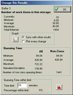
Buffers (also called storage bins or queues) typically collect two types of results, time in queue and queue length. For lean initiatives, the minimum time in the queue is of particular interest as this represents the amount of time that can be eliminated from the system without affecting the downstream operation. This also represents the improvement in total cycle time that is possible. Alternatively, minimum inventory level represents the number of units of inventory that could be eliminated without affecting downstream operations.
|
Figure 1 |
|
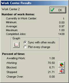
Work centers are active objects that pick up an entity and process it for a (possibly random) processing time. Work centers produce utilization statistics including time spent waiting for work, working, blocked, stopped, and changeover time. If a utilization statistic relates to a bottleneck operation, any time spent waiting for work represents scheduling inefficiencies and an opportunity for improvement. For non-bottleneck operations, non-utilized time represents idle capacity that could be eliminated without affecting the overall system’s output (lean initiatives (Moore and Scheinkopf)). The blocked statistic represents the percentage of time in which a work center is prevented from discharging its completed items due to a limited downstream inventory capacity.
|
Figure 2 |
|
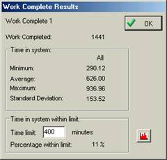
SIMUL8’s work exit point objects are used to mark the removal of an entity from the modeled system, perhaps to represent that a finished good has left the manufacturing facility. Work exit points collect a very useful statistic for lean manufacturers - time in system. This represents the total cycle time for an item from start to finish. An example of this would be the time from when a customer places an order to the time it is delivered. Minimizing this result is another common goal of lean manufacturing.
|
Figure 3 |
|
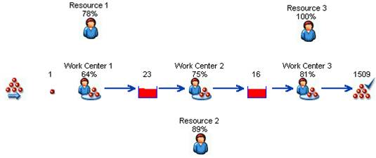
3.1.3 Example – Maximum Buffer Size
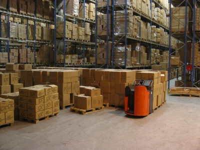
Figure 4 shows a simple simulation model of a 3-work center, 2-buffer operation where work is processed in sequence (Work Center 1, Work Center 2, Work Center 3). The model is used to demonstrate how important buffering is to the performance of a system. Without adequate work-in-process, work centers 2 and 3 may become starved for material and lose precious production time. However, because work center 3 is the bottleneck operation (having the longest process time), work centers 1 and 2 have the potential to continually build inventory.
|
Figure 4 |
|
Specifically, this simple example model above takes into account the following random and dynamic elements:
- Variable process times (Table 1)
- Reliability parameters (Table 1)
- Staggered labor schedules for each machine (Table 2)
|
Table 1 |
|
Process Time |
MTBF |
MTTR |
||
|
|
(minutes) |
Average |
St. Dev. |
Average |
Average |
K |
|
|
Work Center 1 |
8 |
2 |
200 |
45 |
15 |
|
|
Work Center 2 |
9 |
2 |
200 |
45 |
15 |
|
|
Work Center 3 |
10 |
2.5 |
200 |
45 |
15 |
|
Table 2 |
|
Work Center 1 |
Work Center 2 |
Work Center 3 |
|||
|
|
Start |
End |
Start |
End |
Start |
End |
|
|
Shift 1 |
00:00 |
03:00 |
00:30 |
03:30 |
01:00 |
04:00 |
|
|
03:15 |
06:00 |
03:45 |
06:30 |
04:15 |
07:00 |
||
|
06:30 |
08:00 |
07:00 |
08:30 |
07:30 |
09:00 |
||
|
Shift 2 |
08:00 |
11:00 |
08:30 |
11:30 |
09:00 |
12:00 |
|
|
11:15 |
14:00 |
11:45 |
14:30 |
12:15 |
15:00 |
||
|
14:30 |
16:00 |
15:00 |
16:30 |
15:30 |
17:00 |
||
|
Shift 3 |
16:00 |
19:00 |
16:30 |
19:30 |
17:00 |
20:00 |
|
|
19:15 |
22:00 |
19:45 |
22:30 |
20:15 |
23:00 |
||
|
22:30 |
00:00 |
23:00 |
00:30 |
23:30 |
01:00 |
||
The purpose of this model is to investigate the effects of the dynamic and random elements in an effort to impose maximum buffer constraints. By setting maximum buffer sizes, work centers 1 and 2 will be prevented from working. Using simulation, we can vary capacity limitations to investigate the effects on throughput, cycle time, and utilization. For example, Figure 4 is a screen capture of the simulation model at the conclusion of one scenario. The results of this simulation show a total production of 1509 units in 14 days.
In studying simulation models, it has traditionally been necessary to vary the parameters manually from one scenario to the next. Each scenario required a trial of several runs. Results from various scenario trials were then collected and compared to find good quality solutions. Finding an optimal solution could be a laborious, if worthwhile, exercise. With recent advances in simulation optimization algorithms, it is now possible to automate the search for high quality solutions. Companion products are now available for use with simulation languages that allow you to specify an allowable range for input parameter values, as well as a metric for judging the quality of the solution. In our example models, we have chosen to use one such companion product, called OptQuest™ for SIMUL8.
Using OptQuest, we were able to determine the combination of buffer capacities to (1) maximize production and (2) minimize work-in-process. Table 3 shows the total production output for the combination of buffer sizes ranging from 5 to 12 units for Buffer 2 and 18 to 27 units for Buffer 3. The maximum possible production levels are highlighted. Therefore, a buffer combination of 10 and 26 or 9 and 27 will minimize inventory while ensuring maximum production is met. Buffers any larger will not increase production past 1516 but will simply increase cycle time and inventory costs.
|
Table 3 |
|
||||||||||||||||||||||||||||||||||||||||||||||||||||||||||||||||||||||||||||||||||||||||||||||||||||||||||||||||
We intend this example to demonstrate the power of simulation on even a small problem with only a few random elements. Without simulation, it would be very difficult, if not impossible, to determine inventory rules that would meet the same objectives.
Application Areas
The applicability of simulation to various areas or problems is quite remarkable. Almost any process or activity could benefit from simulation, from simple queuing systems to complex manufacturing processes. Below is an overview of the range of simulation applications we have been involved in.
Industries
Although simulation’s roots are in manufacturing, specifically assembly lines, its use is extremely widespread. Application areas include, but are certainly not limited to, the industries show in Table 4.
|
Table 4 |
Manufacturing |
Food and beverage |
Military |
Service industries |
|
Distribution and transportation |
Insurance and banking |
Healthcare |
Mining |
|
|
Forestry |
Entertainment |
Automotive |
Electronics |
|
|
Chemical processing |
Telecommunications |
Education |
Government |
Areas within the Organization
Just as there are many industries, there are many areas within an organization in each industry. These stretch the entire span of an organization’s many activities including marketing, procurement, shop floor manufacturing, inventory management, order fulfillment, and customer service. Each area will certainly have its own unique issues, but many of the principles will remain the same. Any situation in which demand and capacity must be balanced is well-suited to simulation. This may also include the operating rules and management decisions that go into a process.
Examples of Lean Simulations
As we have indicated, simulation is extremely well-suited as a tool for lean manufacturing initiatives. The following are a few examples of how simulation is being used to assist organizations in becoming lean.
Supply Chain
Supply chain analysis is particularly well-suited to simulation because of the interaction of many uncertain and random events. This type of analysis is also commonly targeted by lean advocates because of the high visibility that inventory has within a supply chain. Common elements in supply chains that make it particularly well-suited to simulation include:
|
|
|
|
|
|
|
|
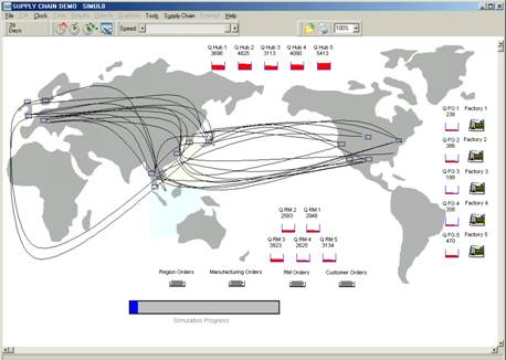
Figure 5 displays a screen shot of a simple supply chain model. In this example, dynamic inventory quantities, including both raw materials and finished goods, are tracked and displayed over time. Incorporating variable lead times, customer demand patterns and inventory management policies, the model allows decision makers to understand how changes in policies are expected to affect inventory build-up.
|
Figure 5 |
|
Implementing KanBan Systems
Kanban is a parts-movement system that assists just-in-time production by moving goods from one workstation to another on a production line. Simulation is not only well suited to determining the feasibility of a kanban system but will also assist in determining the configuration and the number of kanbans required to meet production levels while minimizing inventory.
CNC Horizontal Machining Center
Processes that are reliant on product specific tooling become quite interesting as a balance must be struck between product variety and low work-in-process levels. If a system must rotate between products because of the limited availability of tooling, then many small batches may be preferable to fewer large batches. This is common in computer numerical control (CNC) equipment where tooling racks are product specific. This is even more evident when the variation in process times between products is large.
Case Study - FlexFab Inc.
In manufacturing, there is a constant need to balance the trade-off between minimizing work-in-process inventory and maximizing production efficiency. Figure 6 depicts a production process that serves as an excellent example of this trade-off. The process shown is used to manufacture over 600 different SKUs, some of which are high volume items, others specialty goods. Some stages of the production process can significantly benefit from larger production runs of the same product while others stages are hindered tremendously by the lack of product variety.
At the first stage in the process (extrusion), raw material is converted into an intermediate product in tube form. The tube material is flexible enough to be placed on spools for transporting, protecting, and storing the intermediate product. There are approximately 60 intermediate products of varying size and composition. The spools (small and large), because of their limited availability, act as a type of Kanban to the system. The extrusion process is marred by a significant changeover requirement where changeovers can consume upwards of 50% of the machine’s available time. Therefore, to increase the efficiency of the extrusion process, large production runs of the same, or similar, products would be preferable.
The second operation (cutting), is a manual operation by which the intermediate product is cut to product-specific lengths to meet the production needs of the annealing phase. Once again, large production runs of the same material would save time and increase the efficiency of the cutting operation.
|
Figure 6 |
|
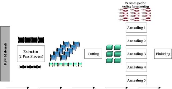
However, at the annealing operation, each of the 600+ products requires unique tooling to hold the item in place during the annealing process. Therefore, in order to support large production runs, there would need to be a very large inventory of tools. Due to the capital cost of the tools, tool purchasing is kept to an absolute minimum. To maximize the utilization of the annealing ovens, operators combine a wide variety of parts (each with their own tooling) to make full loads.
Table 5 summarizes the drivers for efficiency in each production step. Notice that the annealing stage’s driver is completely opposite to the drivers for extrusion and cutting. Annealing would rather see an extremely large variety of products held in work-in-process. Therefore, in order to minimize work-in-process inventory levels, pressure is placed on extrusion and cutting for small production runs.
|
Table 5 |
Operation |
Efficiency Driver |
|
|
Extrusion |
Large Production Runs |
|
|
Cutting |
Large Production Runs |
|
|
Annealing |
Large variety of products in work-in-process |
Simulation is an excellent tool for investigating a system such as this. The management uses simulation to analyze the following aspects of this system:
- Trade off between large and small batches
- Change-over requirements of the extruder
- Effect of the forecasted order book
- Capital expenditures for tooling
- Resulting inventory levels
- Capital expenditure on spools to support increased inventory
- Staffing requirements
Adopting Simulation as a Tool
Simulation is now easier than ever to adopt as a tool within any organization. Reduced cost, improved usability, a shallower learning curve, components (reusable objects), templates (pre-built simulations), and the availability of support services all support the growth in simulation’s popularity and rate of adoption.
Prerequisite Knowledge
Although simulation is easier than ever, we have identified a number of supporting skills required to undertake successful simulation projects.
- Analytical and logical thinking
- Spreadsheet savvy
- Familiarity with basic statistical concepts
- Basic computer programming skills
- Project management skills
For an excellent review of the ideal skills set, please see Rohrer and Banks’ article “Required Skills of a Simulation Analyst”.
Software
There are more simulation vendors than ever before, with a wide rage of solutions available. Table 6 contains a partial list of software vendors with leading edge products ranging in price from several hundred to tens of thousands of dollars. For a survey of software solutions, you may wish to consult http://www.lionhrtpub.com/orms.
|
Table 6 |
Brooks Automation |
CACI Products Company |
Delmia Corp. |
|
|
Flexsim Software Products |
Frontstep, Inc |
Imagine That |
|
|
Lanner Group |
Micro Analysis and Design |
Minuteman Software |
|
|
Orca Computer |
Promodel Corporation |
Rockwell Software |
|
|
SIMUL8 Corp. |
Simulation Dynamics |
XJ Technologies |
Training/Reference Materials
Most software vendors offer training and consulting services to support their products. You will also find a number of professional service companies who specialize in simulation. Many of these companies are independent of the software vendors and support a number of software products. There are a number of annual conferences that attract a wide range of simulation professionals. Two you may wish to attend include: IIE’s Simulation Solutions conference (www.simsol.org) or the Winter Simulation Conference (www.wintersim.org)
Conclusion
Lean manufacturing initiatives target the reduction of unnecessary inventory within a process or organization. This paper outlined many of the reasons that inventory may be required in a system including buffering random elements and dynamic interaction. Simulation is extremely well-suited as a tool to assist managers in assessing the correct inventory levels necessary to absorb the natural variation within any system.
Biographical Sketch
Jaret Hauge is the co-founder and Chief Technical Officer of NovaSim, a simulation services and consulting company headquartered in Bellingham, WA. Before co-founding NovaSim, Jaret headed the technical support, consulting services, and product sales for SIMUL8 while working at Visual Thinking International. He holds a Master of Applied Science in Operations Research from the University of Waterloo and a Bachelor of Commerce degree from the University of Alberta. Jaret’s primary focus at NovaSim is in the development of simulation-based decision support applications.
Kerrie Paige is the president and co-founder of NovaSim. After earning a B.S., Summa Cum Laude, from the University of Puget Sound in Mathematics, an M.S. in Applied Mathematics and a Ph.D. in Operations Research from the University of Colorado at Boulder, Kerrie owned a successful consulting company specializing in computer simulation, optimization, and statistical analysis. Now, with over fifteen years of applied modeling experience, her primary focus is in the development of discrete-event simulation models and the statistical analysis of input and output data.
References
- Hauge, J and Paige, K. 2002. “Learning SIMUL8: The Complete Guide”, PlainVu Publishing, ISBN 09709384-1-1.
- Moore, R and Scheinkopf, L. 1998. “Theory of Constraints and Lean Manufacturing: Friends or Foes”, Chesapeake Consulting Inc.
- Narayanaswamy, R. 2002. “Strategic Layout Planning and Simulation for Lean Manufacturing A LAYOPT™ Tutorial”, Production Modeling Corporation.
- Rohrer, M. and Banks, J. "Required Skills of a Simulation Analyst," IIE Solutions, May, 1998.
 NovaSim